Credit Risk Modelling Simplified: A Look at Probability of Default (PD) Models

Overview of Credit Risk Modelling

Ever Heard of Credit Risk? No worries, we’ve got you covered!

Let’s face it, lending money can be risky. There’s always that chance the person you lend to might not pay you back. This risk of someone defaulting on a loan is what we call credit risk.

Financial markets can be a bit wild sometimes, with their ups and downs. These crazy swings can make it even tougher to predict if someone will repay their loan. Because of this, it’s more important than ever to have good tools to figure out this risk.

Over a decade ago, a set of rules called the Basel II Accord was created. Imagine it as a rulebook for banks, making sure they have a safety net in case of unexpected loan losses. These rules allow some banks to develop their own special models to assess this risk.

These models take a deep dive into three key factors:

1. Chance of Default (PD): This is basically how likely it is that someone won’t repay their loan. Think of it like a guessing game — what are the odds that someone won’t pay you back?
2. Loss Given Default (LGD): If someone skips out on a loan, how much money do you really lose? Imagine selling their stuff to get some money back — this is how much you might get back after selling everything.
3. Exposure at Default (EAD): This is the total amount of money someone owes you if they don’t repay their loan. It’s basically the entire loan amount they borrowed.

By taking these three factors into account, banks can build better models to understand their risk and make sure they have a financial cushion for unexpected loan losses.

Regulatory Environment

Imagine you lend money to a friend. There’s always a chance they might not pay you back, right? That risk of someone defaulting on a loan applies to banks too, only on a much larger scale.

The financial system relies on trust. People need to know their money is safe in the bank. That’s why there are strict rules in place, set by international committees, to make sure banks don’t take on too much risk.

Building the Fortress: The Basel Accords

Think of the Basel Accords as the ultimate rulebook for bank safety. These guidelines dictate how much money banks need to set aside as a buffer against unexpected loan losses. The first version, Basel I, was a basic framework. As the financial world got more complex, so did the rules.

Enter Basel II: Three Pillars for a Stronger System

Basel II introduced a more sophisticated approach built on three key pillars:

• Pillar 1: Minimum Capital Requirements This pillar refines the concept of capital requirements from Basel I. It allows banks to use different methods to calculate their capital needs based on the riskiness of their loans. Here’s how they assess risk:

1. Chance of Default (PD): How likely is it someone won’t repay their loan?
2. Loss Given Default (LGD): If someone defaults, how much money will the bank actually lose?
3. Exposure at Default (EAD): The total amount of money someone owes the bank if they don’t repay.

By considering these factors, banks can build better models to understand their risk and set aside the necessary funds for potential losses using the Expected Loss (EL) formula:

* **EL = PD × LGD × EAD**

For example, let’s say a bank estimates a loan has a 2% chance of default (PD), a potential loss of 40% of the loan amount if it defaults (LGD), and the total loan amount is $10,000 (EAD). The Expected Loss for this loan would be:

* **EL = 0.02 (PD) × 0.4 (LGD) × $10,000 (EAD) = $80**

• Pillar 2: Supervisory Review Process This pillar focuses on regulators working with individual banks to ensure they have strong risk management practices in place. It goes beyond simply meeting the minimum capital requirements and considers a bank’s overall risk profile.
• Pillar 3: Market Discipline This pillar encourages transparency. Banks are required to disclose more information about their risk profiles to the public. This allows investors and depositors to make informed decisions about where to put their money, further incentivizing responsible risk management by banks.

Beyond the Expected: Unexpected Loss (UL): Expected Loss provides a valuable estimate, but it doesn’t account for every possibility. Unexpected Loss (UL) goes beyond the average and considers the potential for more severe losses in extreme scenarios like economic downturns or unforeseen events.

Introducing Risk-Weighted Assets (RWA): Not All Loans Are Created Equal

Now, let’s talk about Risk-Weighted Assets (RWA). This concept is fundamental to Basel II and beyond. RWA considers the riskiness of a bank’s assets, specifically loans. Not all loans are created equal. A government bond carries much less risk than a loan to a high-risk borrower.

Here’s the formula for calculating RWA:

• RWA = Risk Weight × Exposure Amount

Where:

• RWA = Risk-Weighted Asset
• Risk Weight = A percentage assigned by regulators based on the riskiness of the asset (e.g., government bonds might have a 20% risk weight, while high-risk loans might have a 150% risk weight)
• Exposure Amount = The total amount of money owed to the bank by the borrower

Basel II and Risk-Weighted Assets

By using RWAs, Basel II allows banks to calculate their capital requirements more precisely. Banks with a higher proportion of risky assets (higher RWAs) need to hold more capital as a buffer compared to banks with a lower risk profile. This ensures that all banks have adequate reserves to absorb potential losses.

Basel III: Even Stronger Safeguards

Following the 2008 financial crisis, Basel III emerged, building on the foundation of Basel II. It requires banks to hold even more capital as a buffer, especially during economic downturns. This ensures they have the resources to weather financial storms and keep lending money even in tough times.

The Bottom Line: Peace of Mind and a Stable Financial Future

Credit risk regulations might seem complex, but they play a crucial role in safeguarding your money. By setting clear guidelines for banks, the Basel Accords promote a healthy and stable financial system. This stability benefits borrowers too, as it allows banks to continue offering loans at competitive rates.

Development of a Probability of Default (PD) Model

Overview of Probability of Default

For years, banks have been trying to figure out how likely it is that someone borrowing money (the borrower) won’t pay it back. This is called Probability of Default (PD). It’s like a score that helps the bank guess how risky a loan might be.

Here’s how a borrower might be considered in default (not paying back their loan):

1. The Bank Thinks They Can’t Pay: Maybe the borrower goes bankrupt, which means they legally can’t pay their debts. In this case, even if the bank holds collateral (like a house for a mortgage), it might be difficult to recover all the money.
2. Missed Payments: If a borrower misses loan payments for a long time (usually over 90 days), the bank might consider them in default. This is a big deal because it can hurt the borrower’s credit score and make it harder for them to borrow money in the future.

So, by understanding the PD and these signs of default, banks can make better decisions about who to lend money to and how much to charge for loans. This helps them protect themselves from losing money if someone doesn’t pay back what they owe.

Application Scoring

Ever wonder how banks decide whether to approve your loan application? It’s not just a guessing game! Banks use a sophisticated system called application scoring to assess your creditworthiness.

Imagine you’re applying for a loan. The bank gathers information about you, like your age, income, where you live, and your credit history. This information is similar to what you might give a friend if they were considering lending you money.

Here’s how application scoring works:

1. Data Gathering: The bank collects details from your application and potentially other sources like credit bureaus.
2. Scoring the Data: This information is fed into a scoring model, like a complex formula. Each piece of information might have a specific weight based on its importance for predicting loan repayment.
3. Good vs. Bad Borrowers: The model compares your information to historical data on past borrowers. This data helps the model identify patterns between borrower characteristics and their likelihood of repaying loans. People with similar characteristics to good (non-defaulting) borrowers in the past are more likely to receive a higher score.
4. The Outcome: The scoring model generates a number that represents your credit risk — the chance of you defaulting on the loan.

Benefits of Application Scoring:

• Faster Decisions: Scoring helps automate the approval process, making decisions quicker and more efficient.
• Reduced Bias: Scores rely on objective data, minimizing the risk of human bias in loan decisions.
• Better Risk Management: By understanding your risk profile, banks can adjust loan terms like interest rates or tailor products to your needs.

Behavioral Scoring

Imagine you borrow money from a bank. The bank uses a score (credit score) to decide if you’re a good borrower (likely to repay) or a bad borrower (might not repay). This credit score is based on your past financial behavior.

Behavioral scoring is similar, but instead of looking at new loan applicants, it focuses on existing customers. Banks track your financial habits over time, like how much credit you use, if you’re ever late on payments, or if you use your overdraft frequently.

Think of it like a report card for your bank account. This report card helps the bank understand your current risk of not paying back your loans. Here’s how it works:

1. Tracking Your Habits: The bank gathers information about your transactions and account activity. This includes things like how much credit you use on your card compared to your limit (credit utilization rate), how many months you’ve been late on payments (arrears), and if you use your overdraft protection.
2. Understanding Your Risk: Based on your past behavior and information like your age and location (demographic data), the bank creates a score for your account. This score reflects how likely you are to default (not repay) on your loans in the future.
3. Keeping an Eye on You: The bank uses this score to create a risk profile for you. This profile helps them constantly monitor your account and identify any changes in your financial behavior that might indicate a higher risk of defaulting.

The benefit of behavioral scoring for banks is that they can proactively manage their risk. If they see a customer’s score increasing (lower risk), they might offer them a higher credit limit. Conversely, if a customer’s score decreases (higher risk), the bank might take steps to protect themselves, like reducing the credit limit or contacting the customer to discuss their situation.

Ultimately, behavioral scoring helps banks make informed decisions about their existing customers and helps them maintain a healthy financial system.

While application and behavioral scoring models share similar development methodologies, a key distinction exists due to the customer lifecycle stage each assesses. Behavioral models focus on existing customers (“in flight”), eliminating the need for reject inference, a technique used in application scoring to account for unapproved applicants.

Developing a PD Model for Application Scoring

About the Dataset

The KGB dataset, though it might sound ominous, is actually a collection of loan information used to help banks understand their risk. Here’s the breakdown:

• Unbalanced Sample: This dataset only includes people whose loans were approved (good accounts). There are no rejected applicants or those who are still waiting for a decision.
• Balancing the Scales: Even though there are only approved loans, the data is weighted to account for the real world. There are many more good accounts (45,000) compared to bad accounts (1,500). By giving more weight (frequency weight of 30:1) to bad accounts, the data analysis considers them more even though they’re fewer.
• Defining “Bad”: In this dataset, a bad account is simply someone who hasn’t made their loan payment in 90 days or more (delinquent).
• Good vs. Bad: There are no in-between options here. If someone isn’t classified as bad (delinquent), they’re automatically considered good.
• The KGB Variable: The data uses a simple variable called “GB” to indicate whether an account is good or bad.

Code

1. Import Libraries and Load Data

import pandas as pd
import numpy as np
import matplotlib.pyplot as plt
import seaborn as sns
from sklearn.model_selection import train_test_split
from sklearn.preprocessing import StandardScaler, OneHotEncoder
from sklearn.linear_model import LogisticRegression
from sklearn.metrics import roc_auc_score, classification_report
from sklearn.compose import ColumnTransformer
from sklearn.pipeline import Pipeline
from sklearn.impute import SimpleImputer
from imblearn.over_sampling import SMOTE

# Load the data
data = pd.read_csv('KGB.csv')

# Display the first few rows of the dataset
data.head()

2. Handle Missing Values and Categorical Data

Identifying categorical and numerical columns helps us preprocess them accordingly. We impute missing values for numerical data using the median and for categorical data using the most frequent value. Then, we one-hot encode the categorical variables to convert them into a numeric format.

# Identify categorical and numerical columns
categorical_cols = data.select_dtypes(include=['object']).columns
numerical_cols = data.select_dtypes(include=['number']).columns

# Ensure 'GB' is included in the numerical columns
numerical_cols = numerical_cols.drop('GB')

# Impute missing values
imputer = ColumnTransformer([
    ('num', SimpleImputer(strategy='median'), numerical_cols),
    ('cat', SimpleImputer(strategy='most_frequent'), categorical_cols)
])

# Apply imputation and create a DataFrame
data_imputed = imputer.fit_transform(data)
data_imputed = pd.DataFrame(data_imputed, columns=numerical_cols.tolist() + categorical_cols.tolist())

# One-hot encode categorical variables
encoder = OneHotEncoder(drop='first', sparse=False)
encoded_data = encoder.fit_transform(data_imputed[categorical_cols])
encoded_df = pd.DataFrame(encoded_data, columns=encoder.get_feature_names_out(categorical_cols))

# Combine numerical and encoded categorical data
data_preprocessed = pd.concat([data_imputed[numerical_cols], encoded_df], axis=1)

# Add the target variable 'GB'
data_preprocessed['GB'] = data['GB']

3. Outlier Detection and Filtering

Outliers can skew the model’s performance. We use the Interquartile Range (IQR) method to detect and remove outliers from our dataset.

def remove_outliers(df, column):
    Q1 = df[column].quantile(0.25)
    Q3 = df[column].quantile(0.75)
    IQR = Q3 - Q1
    lower_bound = Q1 - 1.5 * IQR
    upper_bound = Q3 + 1.5 * IQR
    return df[(df[column] >= lower_bound) & (df[column] <= upper_bound)]

for col in numerical_cols:
    data_preprocessed = remove_outliers(data_preprocessed, col)

# Check the shape of the dataset after removing outliers
data_preprocessed.shape

4. Data Partitioning

We split the data into training and testing sets. This is crucial for evaluating the model’s performance on unseen data.

X = data_preprocessed.drop('GB', axis=1)
y = data_preprocessed['GB']

X_train, X_test, y_train, y_test = train_test_split(X, y, test_size=0.3, random_state=42, stratify=y)

# Display the shape of the training and testing sets
X_train.shape, X_test.shape

5. Transforming Input Variables

Standardizing the features ensures that they have a mean of zero and a standard deviation of one. This is important for models like logistic regression.

scaler = StandardScaler()
X_train_scaled = scaler.fit_transform(X_train)
X_test_scaled = scaler.transform(X_test)

6. Variable Classing and Selection

We use Logistic Regression with L1 regularization (Lasso) to select the most relevant features. L1 regularization forces the less important feature coefficients to be zero.

# Logistic Regression with L1 regularization
model = LogisticRegression(penalty='l1', solver='liblinear', random_state=42)
model.fit(X_train_scaled, y_train)

# Get the model coefficients
coefficients = pd.Series(model.coef_[0], index=X.columns)

# Select features with non-zero coefficients
selected_features = coefficients[coefficients != 0].index
X_train_selected = X_train[selected_features]
X_test_selected = X_test[selected_features]

# Scale the selected features
X_train_selected_scaled = scaler.fit_transform(X_train_selected)
X_test_selected_scaled = scaler.transform(X_test_selected)

7. Modelling and Scaling

We refit the logistic regression model using the selected features and predict probabilities.

# Re-fit the model with selected features
model = LogisticRegression(random_state=42)
model.fit(X_train_selected_scaled, y_train)

# Predict probabilities
y_train_pred = model.predict_proba(X_train_selected_scaled)[:, 1]
y_test_pred = model.predict_proba(X_test_selected_scaled)[:, 1]

# Scale the probabilities
scaler_prob = StandardScaler()
y_train_pred_scaled = scaler_prob.fit_transform(y_train_pred.reshape(-1, 1))
y_test_pred_scaled = scaler_prob.transform(y_test_pred.reshape(-1, 1))

8. Model Validation

Evaluate the model performance using metrics like ROC-AUC score and classification report.

# ROC-AUC score
train_auc = roc_auc_score(y_train, y_train_pred)
test_auc = roc_auc_score(y_test, y_test_pred)
print(f"Train AUC: {train_auc:.2f}")
print(f"Test AUC: {test_auc:.2f}")

# Classification report
print("Classification Report (Test Data):")
print(classification_report(y_test, model.predict(X_test_selected_scaled)))

9. Reject Inference (concept only)

While our code builds a credit risk model using the KGB dataset (containing only approved loans), it doesn’t account for selection bias. This bias arises because the model is trained solely on good borrowers, excluding rejected applicants (potential bad borrowers).

Reject inference offers a solution. It involves using the current model to score the rejected applications (not included in KGB.csv). These scores can then be used to classify the rejected applications as inferred good or inferred bad borrowers.

The next step would be to create an augmented dataset (AGB). This would involve combining the existing KGB data (good borrowers) with the inferred classifications (good or bad) from the rejected applications. This augmented dataset would represent a more complete picture of the “through-the-door” population (all applicants).

Finally, you could use this augmented dataset (AGB) to train a new credit risk model. This new model would consider both good and inferred bad borrowers, potentially leading to a more accurate prediction of loan defaults.

Generating a Scorecard Report

# Function to transform probabilities into scores
def prob_to_score(prob, base_score=600, pdo=50):
    odds = prob / (1 - prob)
    score = base_score + pdo / np.log(2) * np.log(odds)
    return score

# Apply the function to the predicted probabilities
X_test['PD_Score'] = y_test_pred
X_test['Score'] = X_test['PD_Score'].apply(lambda x: prob_to_score(x))

# Display the test data with predicted scores
print(X_test[['PD_Score', 'Score']].head())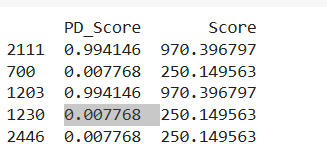

Stay tuned for the next part where we explore the exciting world of Loss Given Default (LGD) models!

Follow me on linkedin

Shorya Sharma | LinkedIn