Credit Risk Modelling Simplified: A Look at Loss Given Default (LGD) Model

What is Loss Given Default (LGD)?
Imagine you’re a lender considering a loan application. LGD helps you estimate the financial blow you might face if the borrower defaults on the loan. It’s expressed as a percentage of the total loan amount outstanding at the time of default. In simpler terms, LGD reflects how much of the loan money you might not be able to recover after selling any collateral that secures the loan.
Why is LGD Important?
LGD is a critical piece of the puzzle in credit risk management. Financial institutions use it along with two other factors, Probability of Default (PD) and Exposure at Default (EAD), to calculate Expected Loss (EL). EL tells you the overall anticipated loss from potential loan defaults within your loan portfolio. By understanding potential losses, lenders can:
- Make informed lending decisions: Accurate LGD estimates allow lenders to set appropriate interest rates and loan terms that manage risk effectively.
- Allocate capital strategically: Knowing the potential losses from different loan types helps banks ensure they have enough reserves set aside to cover defaults.
- Maintain adequate financial buffers: LGD helps determine how much money financial institutions need to set aside to meet their obligations in case of defaults.
LGD Models for Retail Credit
Retail credit refers to loans provided to individuals, such as mortgages, auto loans, and credit cards.
Why are LGD Models Crucial for Retail Credit?
Retail credit portfolios typically hold a large volume of loans with relatively smaller individual loan amounts. While each loan might seem insignificant on its own, defaults across a large portfolio can accumulate to substantial losses. Accurate LGD models become even more critical in this scenario, helping lenders manage risk effectively:
- Fine-Tuning Risk Assessment: LGD models enable lenders to assess the risk profile of each borrower beyond just a credit score. By considering factors like income, employment history, and loan purpose, the model can provide a more nuanced prediction of potential recovery rates in case of default.
- Tailoring Credit Products: Insights from LGD models can inform the creation of credit products with appropriate interest rates and terms that reflect the borrower’s risk profile and the lender’s potential loss exposure.
- Strategic Pricing: LGD models can help lenders price loans competitively while ensuring they cover the expected loss associated with a certain risk profile.
LGD Models for Corporate Credit
Corporate credit deals with loans extended to businesses, ranging from short-term working capital loans to long-term project financing.
Why are LGD Models Essential for Corporate Credit?
Corporate loans often involve larger sums compared to retail credit. While defaults might be less frequent, the potential losses can be significant. LGD models become crucial tools for managing risk in this environment:
- Sophisticated Risk Assessment: Corporate borrowers are complex entities with diverse financial structures and business models. LGD models can incorporate various factors beyond just financial statements, such as industry trends, collateral valuations, and legal frameworks. This allows for a more comprehensive assessment of potential recovery rates in case of default.
- Credit Risk Differentiation: LGD models help differentiate risk profiles within the corporate borrower landscape. This enables lenders to set appropriate interest rates and loan terms that reflect the varying degrees of risk associated with different borrowers.
- Enhanced Capital Allocation: By understanding potential losses from corporate loans, banks can strategically allocate capital reserves. This ensures they have sufficient resources to weather potential defaults within their corporate loan portfolio.
Tailoring LGD Models for Corporate Credit:
Due to the complexities of corporate borrowers, LGD models for corporate credit often employ more advanced techniques compared to retail credit models. Here are some common approaches:
- Loss Forecasting Models: These sophisticated models incorporate time series analysis and economic indicators to predict recovery rates. This allows for a more dynamic assessment that considers how external factors like economic cycles can impact a borrower’s ability to repay.
- Scenario Analysis: LGD models can be used to simulate different default scenarios and their impact on recovery rates. This helps lenders stress-test their portfolios and assess their resilience to various economic or industry downturns.
- Credit Migration Models: These models predict the likelihood of a borrower’s credit quality deteriorating over time. This information can be integrated with LGD models to provide a more comprehensive picture of potential losses throughout the loan lifecycle.
Challenges and Considerations in Corporate LGD Modeling:
Building and maintaining effective LGD models for corporate credit comes with its own set of challenges:
- Data Availability: Obtaining detailed financial and industry-specific data on corporate borrowers can be more complex compared to retail credit.
- Model Complexity: The sophisticated nature of corporate LGD models can require significant expertise to develop and interpret.
- Market Volatility: Corporate default rates and recovery experiences can be more susceptible to fluctuations in the broader economic environment. LGD models need to be adaptable to capture these changing dynamics.
Economic Variables for LGD Estimation
Loss Given Default (LGD) models don’t exist in a vacuum. Economic conditions can significantly impact a borrower’s ability to repay a loan and, consequently, the amount of money recovered in case of default. In this section, we’ll explore some key economic variables that can be incorporated into LGD models to provide a more comprehensive picture of potential losses.
Why Include Economic Variables in LGD Models?
Economic factors create a broader context that influences a borrower’s financial health and recovery prospects. Here’s how economic variables enhance LGD models:
- Improved Accuracy: By considering economic conditions alongside borrower-specific factors, LGD models can provide more accurate estimates of recovery rates in different scenarios.
- Proactive Risk Management: Economic variables can help anticipate potential losses during economic downturns, allowing lenders to take proactive measures like increasing loan loss provisions or tightening credit standards.
- Stress Testing and Scenario Analysis: LGD models that incorporate economic variables can be used for stress testing loan portfolios. This allows lenders to assess their vulnerability to various economic shocks and adjust their risk management strategies accordingly.
Examples of Economic Variables for LGD Estimation:
Here are some key economic variables that can be integrated into LGD models:
- Gross Domestic Product (GDP) Growth: A strong economy generally translates into lower default rates and higher recovery rates. Conversely, a recessionary environment can lead to increased defaults and lower recoveries.
- Unemployment Rate: Higher unemployment rates indicate a weaker job market and potentially lower borrower repayment capacity. This can translate into higher LGD estimates.
- Interest Rates: Changes in interest rates can impact a borrower’s ability to service their debt. Rising interest rates can put additional strain on borrowers, potentially increasing LGD.
- Inflation Rate: Inflation can erode the value of recovered assets, leading to lower LGD estimates. However, high inflation can also lead to increased borrower income, potentially improving repayment capacity.
- Industry-Specific Indicators: For corporate LGD models, incorporating industry-specific economic indicators like commodity prices or sectoral growth rates can provide further insights into a borrower’s risk profile.
Estimating Downturn LGD
While standard LGD models provide valuable insights under normal economic conditions, they might underestimate potential losses during periods of economic downturn. Downturn LGD specifically focuses on estimating these potential losses during economic hardships. Here, we’ll delve into the intricacies of estimating downturn LGD.
Why is Downturn LGD Important?
Economic downturns can significantly increase default rates and decrease recovery rates for loans. Downturn LGD helps lenders prepare for these harsher conditions by:
- Strengthening Capital Adequacy: By estimating higher potential losses during downturns, lenders can ensure they have sufficient capital reserves to absorb these losses and maintain financial stability.
- Informing Risk Management Strategies: Downturn LGD estimates can guide lenders in adjusting their risk management strategies during economic downturns. This might involve tightening credit standards, increasing loan loss provisions, or focusing on loan portfolios less vulnerable to downturns.
- Regulatory Requirements: Many financial regulations require banks to incorporate downturn LGD estimates into their capital adequacy calculations.
Approaches to Estimating Downturn LGD:
There are two main approaches to estimating downturn LGD, each with its own advantages and limitations:
- Type 1: Downturn LGD Calibration Based on Observed Impact: This approach leverages historical data from past economic downturns. It analyzes the impact of those downturns on actual default rates and recovery rates within a specific loan portfolio. This method requires sufficient historical data on past downturns that were relevant to the current loan portfolio characteristics.
- Type 2: Downturn LGD Calibration Based on Estimated Impact: When historical downturn data is limited or not directly applicable, this approach uses statistical techniques and economic forecasts to estimate the impact of a hypothetical downturn on LGD. This method can be more flexible but relies on the accuracy of the chosen estimation techniques and economic forecasts.
Regression Techniques for LGD
Loss Given Default (LGD) models play a vital role in credit risk management, and regression analysis stands as a powerful statistical technique for building these models. This section will delve into the specifics of using regression techniques for LGD estimation.
Why Regression Analysis for LGD Models?
Regression analysis offers a structured and data-driven approach to modeling LGD. Here’s how it shines:
- Quantifying Relationships: Regression analysis helps identify and quantify the relationships between borrower characteristics (independent variables) and LGD (dependent variable). This allows for a more nuanced understanding of how different factors influence potential losses.
- Improved Prediction Accuracy: By leveraging these quantified relationships, regression models can predict LGD for new borrowers based on their characteristics. This enhances the model’s ability to estimate potential losses across a loan portfolio.
- Interpretability: Regression analysis provides coefficients that indicate the direction and strength of the relationship between each borrower characteristic and LGD. This interpretability helps lenders understand which factors have the most significant impact on recovery rates.
Common Regression Techniques for LGD Modeling:
There are several regression techniques used for LGD modeling, each with its strengths and considerations:
- Linear Regression: This is the most basic approach, assuming a linear relationship between borrower characteristics and LGD. It’s easy to implement but may not capture non-linear relationships that might exist in real-world data.
- Logistic Regression: This technique is suitable when LGD is expressed as a probability (between 0 and 1). It’s particularly useful for modeling binary outcomes, such as whether a default will result in a complete loss (LGD of 1) or some recovery (LGD between 0 and 1).
- Beta Regression: This technique is specifically designed for modeling data constrained between 0 and 1, like LGD. It offers more flexibility compared to logistic regression when dealing with the specific distribution of LGD values.
Advanced Regression Techniques for LGD:
As LGD modeling becomes more sophisticated, advanced regression techniques can be employed:
- Random Forest Regression: This ensemble method combines multiple decision trees to create a more robust and accurate model. It can handle complex relationships between variables and is less prone to overfitting.
- Support Vector Regression (SVR): This technique is known for its ability to handle high-dimensional data and non-linear relationships. It can be particularly useful when dealing with a large number of borrower characteristics.
Performance Metrics for LGD
Several metrics are used to assess LGD model performance, each offering insights into different aspects:
- Mean Squared Error (MSE): This metric measures the average squared difference between predicted LGD values and actual LGD values observed in historical data. A lower MSE indicates a better fit between the model’s predictions and reality.
Formula:
MSE = (1/n) Σ (Y_i — Ŷ_i)²
where:
- n is the number of observations (loans)
- Y_i is the actual LGD value for loan i
- Ŷ_i is the predicted LGD value for loan i by the model
- Root Mean Squared Error (RMSE): This metric is the square root of MSE and is expressed in the same units as LGD (e.g., percentage). It provides a more intuitive understanding of the average prediction error.
Formula:
RMSE = √MSE
- Mean Absolute Error (MAE): This metric measures the average absolute difference between predicted LGD values and actual LGD values. It’s less sensitive to outliers compared to MSE and can be useful for assessing model performance across the entire LGD distribution.
Formula:
MAE = (1/n) Σ |Y_i — Ŷ_i|
- Goodness-of-Fit Statistics: These metrics, like R-squared (linear regression) or McFadden’s R-squared (logistic regression), indicate how well the model explains the variation in LGD observed in the data. A higher R-squared value suggests a better fit.
Additionally, for LGD models that predict the entire LGD distribution, other graphical tools can be employed for evaluation:
- QQ Plots (Quantile-Quantile Plots): These plots compare the distribution of predicted LGD values with the distribution of actual LGD values. A good fit suggests the model is capturing the LGD distribution accurately.
- KS Statistic (Kolmogorov-Smirnov Statistic): This metric measures the maximum difference between the cumulative distribution functions of predicted and actual LGD values. A lower KS statistic indicates a better alignment between the two distributions.
Case Study
Case Study: Loss Estimation for CNB Bank
About Company:
CNB Bank provides various car loans to customers. The bank needs to estimate potential losses in case customers default on their loans. They want to automate this estimation process using customer details provided at the time of loan application.
Problem: The bank wants to automate the loss estimation based on customer detail provided while applying for loan. These details are Age, Years of Experience, Number of cars, Gender, Marital Status. To automate this process, they have given a problem to identify the loss estimation given that the customers is a defaulter, those are eligible for loan amount so that they get to know what features are leading to defaults upto which amount. Here are the details about the data set.

Get The dataset from : ML_Sklearn/LGD_DATA.csv at master · shorya1996/ML_Sklearn (github.com)
Code:
import pandas as pd
import numpy as np
from sklearn.model_selection import train_test_split
from sklearn.preprocessing import StandardScaler, LabelEncoder
from sklearn.linear_model import LinearRegression
from sklearn.metrics import mean_squared_error, r2_score
import matplotlib.pyplot as plt
import seaborn as sns

# Load the dataset
file_path = 'LGD_DATA.csv'
data = pd.read_csv(file_path)

# Display the first few rows of the dataset
print("First few rows of the dataset:")
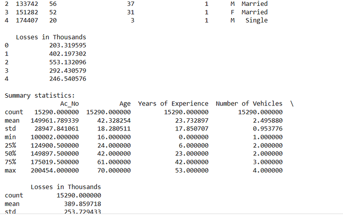
print(data.head())

# Display summary statistics of the dataset
print("\nSummary statistics:")
print(data.describe())

# Display information about the dataset
print("\nDataset info:")
print(data.info())

# Check for missing values
print("\nMissing values in each column:")
print(data.isnull().sum())
import seaborn as sns
#to plot histograms
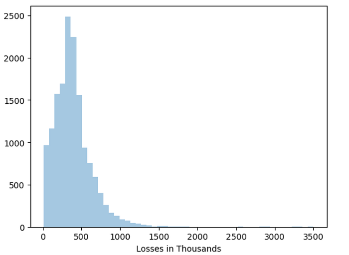
sns.distplot(data['Losses in Thousands'],kde=False,bins=50)
import math
# this probably means we shud take the log to normalize the data
log_losses = np.array(list(map(math.log,data['Losses in Thousands'])))
sns.distplot(log_losses,kde=False,bins=50)
# map function is used to apply any function on each element of a series/list
# now the distribution looks normal
# Convert non-numerical columns to numerical using LabelEncoder
for column in data.columns:
    if data[column].dtype == type(object):
        le = LabelEncoder()
        data[column] = le.fit_transform(data[column])

# Calculate correlations
data.corr()
# we see a high co-relatin between Age and Years of Experience
# which is obvious as with Age your Experience increases
from sklearn.model_selection import train_test_split
from sklearn.preprocessing import StandardScaler, LabelEncoder

# Handle missing values
data = data.dropna()  # Dropping missing values for simplicity
# Encode categorical variables
le_gender = LabelEncoder()
data['Gender'] = le_gender.fit_transform(data['Gender'])

le_married = LabelEncoder()
data['Married'] = le_married.fit_transform(data['Married'])

# Create age categories
data['AgeCategory'] = data['Age'].apply(lambda x: 'Young' if x <= 28 else 'MiddleAged' if x < 58 else 'Old')
age_category_dummies = pd.get_dummies(data['AgeCategory'], drop_first=True)
data = pd.concat([data, age_category_dummies], axis=1)

# Apply log transformation to the target variable to normalize it
data['LogLoss'] = data['Losses in Thousands'].apply(math.log)

# Feature scaling
scaler = StandardScaler()
numerical_columns = ['Age', 'Years of Experience', 'Number of Vehicles']
data[numerical_columns] = scaler.fit_transform(data[numerical_columns])

# Select features and target variable
X = data[['Age', 'Years of Experience', 'Number of Vehicles', 'Gender', 'Married', 'Old', 'Young']]
y = data['LogLoss']

# Split the data into training and testing sets
X_train, X_test, y_train, y_test = train_test_split(X, y, test_size=0.3, random_state=1)

from sklearn.linear_model import LinearRegression
from sklearn.metrics import mean_absolute_error, r2_score
# Model Development
model = LinearRegression()
model.fit(X_train, y_train)

# Predictions and evaluation
y_pred = model.predict(X_test)
mae = mean_absolute_error(y_test, y_pred)
r2 = r2_score(y_test, y_pred)

print(f'Mean Absolute Error: {mae}')
print(f'R^2 Score: {r2}')

# Model coefficients
print('Intercept:', model.intercept_)
print('Coefficients:', model.coef_)
# Visualization of true vs predicted values
plt.figure(figsize=(10, 6))
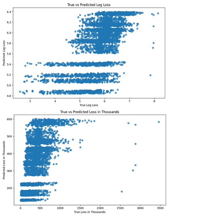
plt.scatter(y_test, y_pred, alpha=0.7)
plt.xlabel('True Log Loss')
plt.ylabel('Predicted Log Loss')
plt.title('True vs Predicted Log Loss')
plt.show()

# Inverse log transformation to compare true loss and predicted loss in original scale
y_test_exp = np.exp(y_test)
y_pred_exp = np.exp(y_pred)

plt.figure(figsize=(10, 6))
plt.scatter(y_test_exp, y_pred_exp, alpha=0.7)
plt.xlabel('True Loss in Thousands')
plt.ylabel('Predicted Loss in Thousands')
plt.title('True vs Predicted Loss in Thousands')
plt.show()
This blog has taken you on a journey into the world of Loss Given Default (LGD) models. We’ve explored how these powerful tools empower lenders to assess potential losses from loan defaults, across both retail and corporate credit landscapes. We’ve delved into regression techniques, downturn LGD considerations, and performance metrics for robust model evaluation.
Are you ready to leverage LGD models to make informed lending decisions and optimize your credit risk management strategy?
Follow me on Linkedin and Instagram
